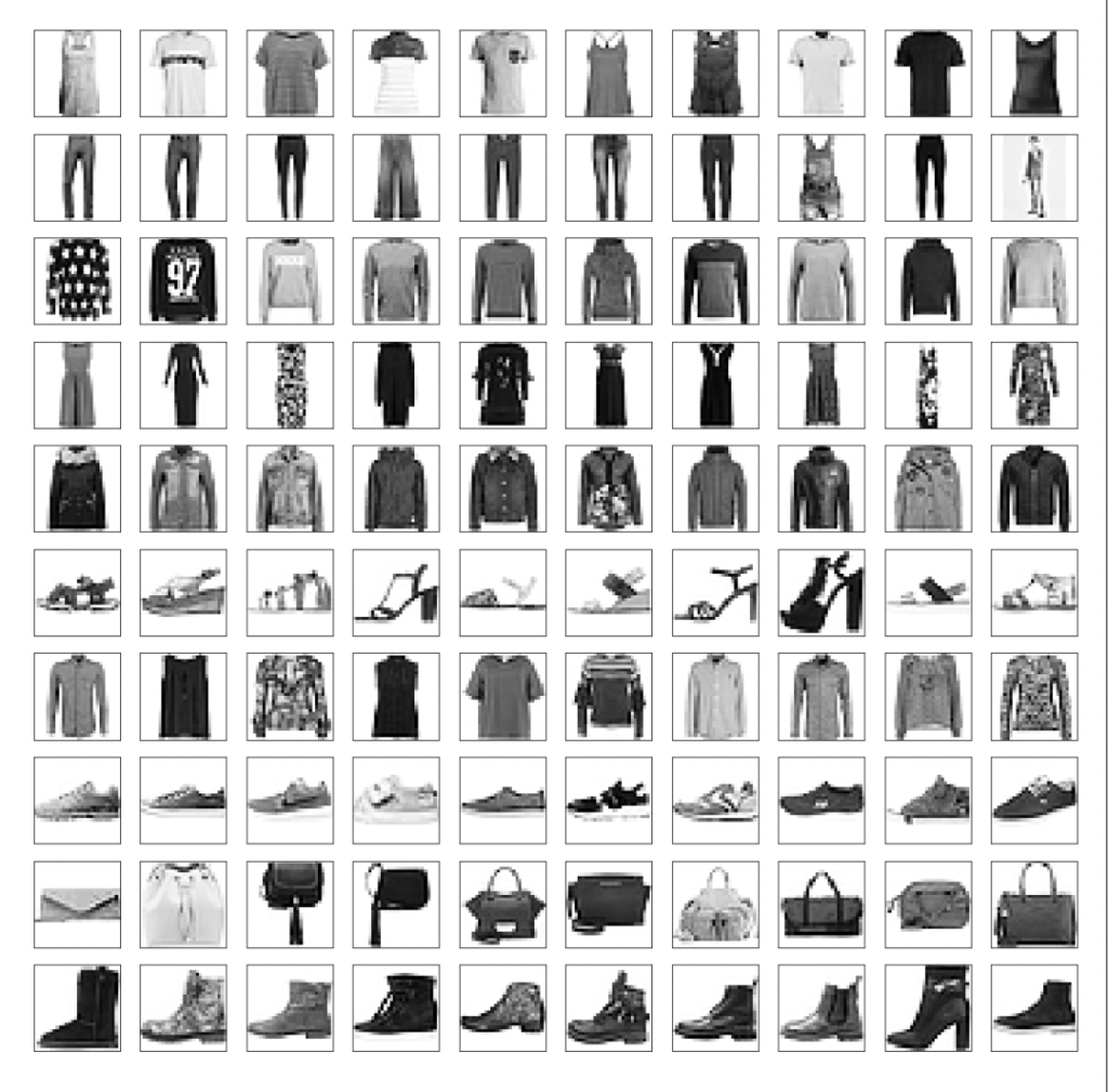
Fashion MNIST Image Classification Using KNN

Fashion-MNIST is a dataset of Zalando’s article images, consisting of a training set of 60,000 examples and a
test set of 10,000 examples. Each example is a 28×28 grayscale image, associated with a label from 10
classes.
Each training and test example is assigned to one of the following labels: T-shirt/top, trousers, Pullover,
Dress, Coat, Sandal, Shirt, Sneaker, Bag, Ankle Boot

Dataset link: https://www.kaggle.com/datasets/zalando-research/fashionmnist

In the CSV file of both train and test set
Each row is a separate image
Column 1 is the class label
The remaining columns are pixel numbers (784 total)
Each value is the darkness of the pixel (1 to 255)
Aim: To build a classification model using the KNN algorithm to identify correct labels based on the images

#importing libraries to perform EDA
import numpy as np
import pandas as pd
import matplotlib.pyplot as plt
import seaborn as sns
import warnings
warnings.filterwarnings('ignore')

# reading the data csv and converting it into a dataframe
df=pd.read_csv('./fashion-mnist_train.csv')
# quick peek into the dataframe
df.head()

# checking the datatypes in this dataframe
df.info()
# checking for null-values
df.isnull().sum().sum()

# checking the number of duplicated images
df.duplicated().sum()


# dropping the above 43 duplicated images
df.drop_duplicates(inplace=True)
df.shape

df.label.unique()

# lets now analyze the labels and their corresponding numbers
colors = sns.color_palette('mako_r')[1:3]
plt.pie(x=df.groupby(['label']).count()['pixel1'],labels=df.groupby(['label']).count().index)

Data Preprocessing & Making Pipeline

from sklearn.pipeline import Pipeline
from sklearn.preprocessing import MinMaxScaler
from sklearn.model_selection import cross_validate
from sklearn.neighbors import KNeighborsClassifier

# Creating X and y variables
X=df.drop('label',axis=1)
y=df.label

xx=X[0:500]
yy=y[0:500]

Due to the large amount of data we are just taking 500 samples to train the model.

# instantiating normalizer object
normalize=MinMaxScaler()

Here we are creating different models for different values of K, in order to find the optimal value of K using
elbow graph

test_error_rate=[]
train_error_rate=[]
for k in range(1,31):
    # creating a KNN model with K
    knn=KNeighborsClassifier(k)
    # sequence of operations to be performed
    operations=[('normalize',normalize),('knn',knn)]
    # creating a pipeline
    pipe=Pipeline(steps=operations)
    # performing 5-fold cross validation using the pipeline and df
    cross_dict=cross_validate(pipe,xx,yy,cv=5,scoring='accuracy', return_train_score=True)
    # capturing train and test error rate for elbow graph
    test_error_rate.append(cross_dict['test_score'].mean())
    train_error_rate.append(cross_dict['train_score'].mean())

train_error_rate=[1-acc for acc in train_error_rate]
test_error_rate=[1-acc for acc in test_error_rate]

Plotting the elbow-graph to figure the optimal value K

plt.title('Elbow Graph')
plt.xlabel('K')
plt.ylabel('error_rate')
sns.lineplot(x=range(1,31),y=test_error_rate, color='red');

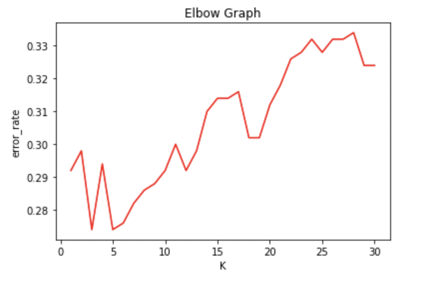
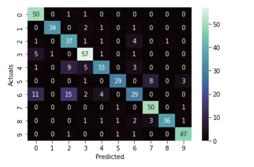
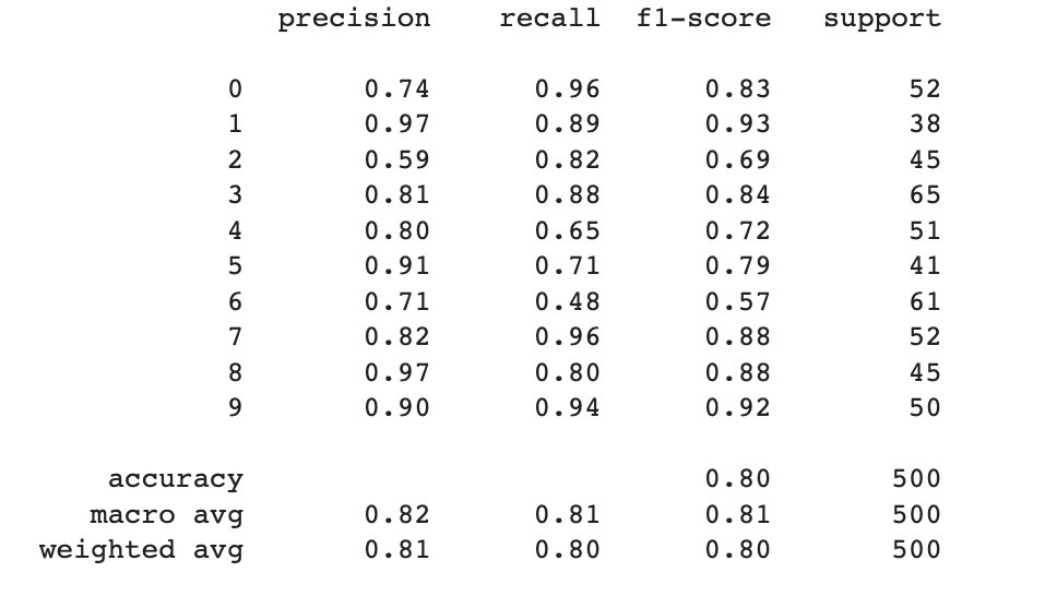
From the above elbow graph, we see that the test error rate is lowest when K=5. Let us now build our final model using this value of K and then obtain the confusion matrix and complete classification report for both the training set (here the entire df is the training set) and the testing set (which is a totally unseen dataset, yet to be imported)

Building Final Model: KNN

# instantiating a knn object with K=5
knn=KNeighborsClassifier(n_neighbors=5)

# normalizing the predictors
X_norm=normalize.fit_transform(xx)

# fitting the transformed data on the above KNeighborsClassifier object
knn.fit(X_norm,yy)

# making predictions off of the dataset using the above KNN model
y_pred=knn.predict(X_norm)
y_pred

Evaluation Matrxis

from sklearn.metrics import confusion_matrix, classification_report, accuracy_score

# creating confusion matrix for this training set
sns.heatmap(confusion_matrix(yy,y_pred), annot=True, cmap='mako', fmt='.5g')
plt.xlabel('Predicted')
plt.ylabel('Actuals')

print(classification_report(yy,y_pred))

# computing the exact accuracy_score
train_accuracy=round(100*accuracy_score(yy,y_pred),2)
print(f'The train accuracy score is {train_accuracy}%')

#reading the data csv and converting it into a dataframe
df_test=pd.read_csv('./fashion-mnist_test.csv')
#quick peek into the dataframe
df_test.head()

# checking the datatypes in this dataframe
df_test.info()

# checking for null-values
df_test.isnull().sum().sum()

# splitting the testing set into predictor and target variables
X_test=df_test.drop('label',axis=1)
y_test=df_test.label


# normalizing the predictors using the same scaling object. We're applying only transform h
X_test_norm=normalize.transform(X_test)

# making predictions off of the testing data using the same knn model
y_test_pred=knn.predict(X_test_norm)

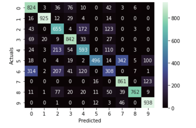
# creating confusion matrix for this testing set
sns.heatmap(confusion_matrix(y_test,y_test_pred), annot=True, cmap='mako', fmt='.5g')
plt.xlabel('Predicted')
plt.ylabel('Actuals');

print(classification_report(y_test,y_test_pred))

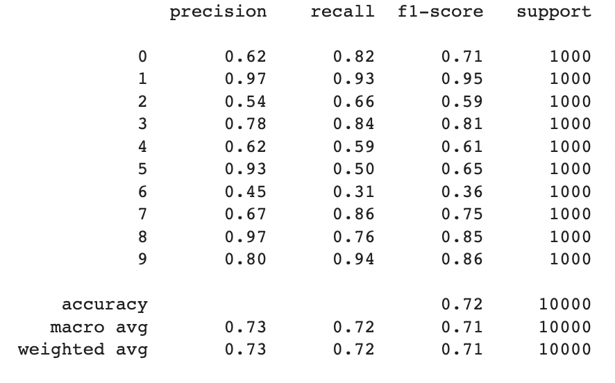
# computing the exact accuracy_score
test_accuracy=round(100*accuracy_score(y_test,y_test_pred),2)
print(f'The test accuracy score is {test_accuracy}%')

Github Link: https://github.com/noumannahmad/Fashion-MNIST-Image-Classification-Using-KNN