Diagnosis for prediction of knee osteoarthritis using deep learning

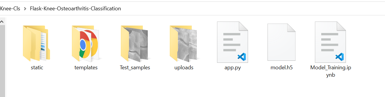
In this blog, we learn how to diagnosis the prediction of X-rays knee classification using Convolutional neural network and then deploy the model using Web-based Flask application.

Diagnosis for the prediction of knee osteoarthritis using deep learning techniques.

The dataset consists of 1650 digital X-ray images of knee joint which are collected from well reputed hospitals and diagnostic centres. The X-ray images are acquired using PROTEC PRS 500E X-ray machine. Original images are 8-bit grayscale image. Each radiographic knee X-ray image is manually annotated /labelled as per Kellgren and Lawrence grades by 2 medical experts. A novel approach has been developed to automatically extract the Cartilage region (region of interest) based on density of pixels. The target is to evaluate the performance of the deep learning algorithm to predict per Kellgren and Lawrence grades.

the Kellgren and Lawrence classification system: grade 0 (normal): definite absence of x-ray changes of osteoarthritis grade 1 (doubtful): doubtful joint space narrowing and possible osteophytic lipping grade 2 (mid): definite osteophytes and possible joint space narrowing grade 3 (moderate): moderate multiple osteophytes, definite narrowing of joint space and some sclerosis and possible deformity of bone ends grade 4 (severe): large osteophytes, marked narrowing of joint space, severe sclerosis and definite deformity of the bone end. 

Dataset link:

https://data.mendeley.com/datasets/t9ndx37v5h/1

Data Preprocessing

import cv2,os
data_path='/content/drive/MyDrive/Knee-project/Knee-Dataset/'
categories=os.listdir(data_path)
labels=[i for i in range(len(categories))]

label_dict=dict(zip(categories,labels)) #empty dictionary
print(label_dict)
print(categories)
print(labels)

img_size=256
data=[]
label=[]

for category in categories:
    folder_path=os.path.join(data_path,category)
    img_names=os.listdir(folder_path)
        
    for img_name in img_names:
        img_path=os.path.join(folder_path,img_name)
        img=cv2.imread(img_path)
        try:
            gray = cv2.cvtColor(img, cv2.COLOR_BGR2GRAY)  
            resized=cv2.resize(gray,(img_size,img_size))
            #resizing the image  into 256 x 256, since we need a fixed common size for all the images in the dataset
            data.append(resized)
            label.append(label_dict[category])
            #appending the image and the label(categorized) into the list (dataset)
        except Exception as e:
            print('Exception:',e)
            #if any exception rasied, the exception will be printed here. And pass to the next image

Recale and assign catagorical labels

import numpy as np
data=np.array(data)/255.0
data=np.reshape(data,(data.shape[0],img_size,img_size,1))
label=np.array(label)
from keras.utils import np_utils
new_label=np_utils.to_categorical(label)

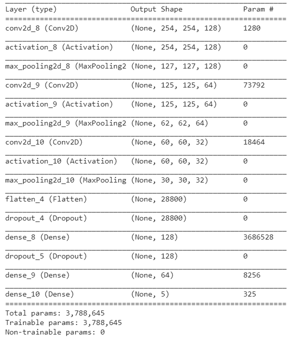
convolutional neural network architectures

from keras.models import Sequential
from keras.layers import Dense,Activation,Flatten,Dropout
from keras.layers import Conv2D,MaxPooling2D
from keras.callbacks import ModelCheckpoint

model=Sequential()

model.add(Conv2D(128,(3,3),input_shape=data.shape[1:]))
model.add(Activation('relu'))
model.add(MaxPooling2D(pool_size=(2,2)))
#The first CNN layer followed by Relu and MaxPooling layers

model.add(Conv2D(64,(3,3)))
model.add(Activation('relu'))
model.add(MaxPooling2D(pool_size=(2,2)))
#The second convolution layer followed by Relu and MaxPooling layers

model.add(Conv2D(32,(3,3)))
model.add(Activation('relu'))
model.add(MaxPooling2D(pool_size=(2,2)))
#The thrid convolution layer followed by Relu and MaxPooling layers

model.add(Flatten())
#Flatten layer to stack the output convolutions from 3rd convolution layer
model.add(Dropout(0.2))

model.add(Dense(128,activation='relu'))
#Dense layer of 128 neurons

model.add(Dropout(0.1))
model.add(Dense(64,activation='relu'))
#Dense layer of 64 neurons

model.add(Dense(5,activation='softmax'))
#The Final layer with two outputs for two categories

model.compile(loss='categorical_crossentropy',optimizer='adam',metrics=['accuracy'])

Splitting data into training and testing

from sklearn.model_selection import train_test_split
x_train,x_test,y_train,y_test=train_test_split(data,new_label,test_size=0.1)

import matplotlib.pyplot as plt
plt.figure(figsize=(10,10))
for i in range(20):
    plt.subplot(5,5,i+1)
    plt.xticks([])
    plt.yticks([])
    plt.grid(False)
    plt.imshow(np.squeeze(x_test[i]))
    plt.xlabel(categories[np.argmax(y_test[i])])
plt.show()

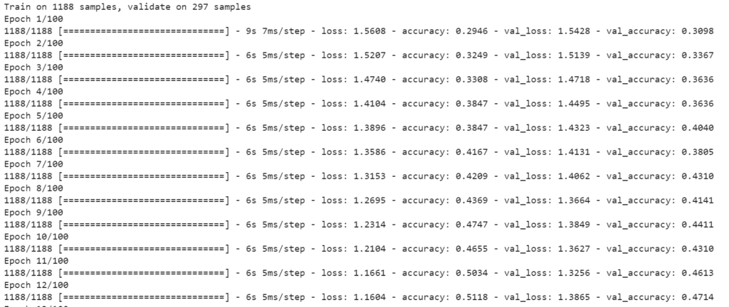
history=model.fit(x_train,y_train,epochs=100,validation_split=0.2)

model.save('model.h5')

from matplotlib import pyplot as plt
# plot the training loss and accuracy
N = 100 #number of epochs
plt.style.use("ggplot")
plt.figure()
plt.plot(np.arange(0, N), history.history["loss"], label="train_loss")
plt.plot(np.arange(0, N), history.history["val_loss"], label="val_loss")
plt.plot(np.arange(0, N), history.history["accuracy"], label="train_acc")
plt.plot(np.arange(0, N), history.history["val_accuracy"], label="val_acc")
plt.title("Training Loss and Accuracy")
plt.xlabel("Epoch #")
plt.ylabel("Loss/Accuracy")
plt.legend(loc="center right")
plt.savefig("CNN_Model")

vaL_loss, val_accuracy= model.evaluate(x_test, y_test, verbose=0)
print("test loss:", vaL_loss,'%')
print("test accuracy:", val_accuracy,"%")

X = 32
img_size = 256
img_single = x_test[X]
img_single = cv2.resize(img_single, (img_size, img_size))
img_single = (np.expand_dims(img_single, 0))
img_single = img_single.reshape(img_single.shape[0],256,256,1)

predictions_single = model.predict(img_single)
print('A.I predicts:',categories[np.argmax(predictions_single)])
print("Correct prediction for label",np.argmax(y_test[X]),'is',categories[np.argmax(y_test[X])])
plt.imshow(np.squeeze(img_single))
plt.grid(False)
plt.show()

from sklearn.metrics import confusion_matrix
from mlxtend.plotting import plot_confusion_matrix

test_labels = np.argmax(y_test, axis=1)
predictions = model.predict(x_test)
predictions = np.argmax(predictions, axis=-1)

cm  = confusion_matrix(test_labels, predictions)
plt.figure()
plot_confusion_matrix(cm,figsize=(12,8), hide_ticks=True,cmap=plt.cm.Blues)
plt.xticks(range(5), ['Normal','Doubtful','Mid','Moderate','Severe'], fontsize=16)
plt.yticks(range(5), ['Normal','Doubtful','Mid','Moderate','Severe'], fontsize=16)
plt.show()

Flask App Interface

Download complete Project: