
An autoencoder is a type of artificial neural network used to learn efficient data codings in an unsupervised manner. The aim of an autoencoder is to learn a representation (encoding) for a set of data, typically for dimensionality reduction, by training the network to ignore signal “noise”.
AutoEncoders compress the input into a lower-dimensional code and then reconstruct the output from this representation. The code is a compact “summary” or “compression” of the input also called the latent-space representation.

Build an autoencoder need three components:
- Encoding method
- Decoding method
- Loss function to compare the output with the target.
The architecture
Both the encoder and decoder are fully connected feed-forward Neural Networks. Code is a single layer with the dimensionality of our choice. The number of nodes in the (Latent Representation )code layer is a hyperparameter that we set before training the autoencoder.
Autoencoders are mainly a dimensionality reduction (or compression) algorithm

The details:
- First, the input passes through the encoder, which is a fully connected ANN, to produce the code. The decoder, which has a similar ANN structure, then produces the output only using this code (latent Representation ).
- The goal is to get an output identical to the input. Note that the decoder architecture is generally the mirror image of the encoder. This is not a requirement but is typically the case.
- The only requirement is the dimensionality of the input and output needs to be the same. Anything in the middle can be played with.
- There are 4 hyper-parameters that we need to set before training an autoencoder:
- Code size (Latent Representation)
- Number of layers
- Loss function
- Number of nodes per layer
Keeping the code layer small can force an AE to learn a low-dimensional intelligent representation of the data.
Denoising AutoEncoders:
There is another way to force the AutoEncoder to learn useful features, and that is – adding random noise to its inputs and making it recover the original noise-free data.

By subtracting the noise and produce the underlying meaningful data. This is called a denoising AutoEncoder. Here random Gaussian noise is added to the AutoEocder and the noisy data becomes the input to the autoencoder.

The bottom row is the AutoEnocder output.
Implementation
Deep inside: Autoencoders
4 types of autoencoders are described using the Keras framework and the MNIST dataset.
- Vanilla autoencoders
- Multilayer autoencoder
- Convolutional autoencoder
- Regularized autoencoder: 1. Sparse Auto Encoder 2. Denoising Auto Encoder
Import the libraries
import keras
import numpy as np
import matplotlib.pyplot as plt
%matplotlib inline

from keras.datasets import mnist
from keras.models import Model
from keras.layers import Input, add
from keras.layers.core import Layer, Dense, Dropout, Activation, Flatten, Reshape
from keras import regularizers
from keras.regularizers import l2
from keras.layers.convolutional import Conv2D, MaxPooling2D, UpSampling2D, ZeroPadding2D
from keras.utils import np_utils
Load the data
Note We don’t need the labels as the autoencoders are unsupervised network.
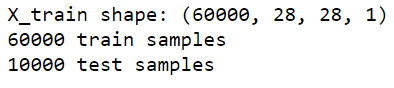
(X_train, _), (X_test, _) = mnist.load_data()

X_train = X_train.reshape(X_train.shape[0], 28, 28, 1)
X_test = X_test.reshape(X_test.shape[0], 28, 28, 1)
Normalize the data
We want the pixels values between 0 and 1 instead of between 0 and 255
X_train = X_train.astype("float32")/255.
X_test = X_test.astype("float32")/255.

print('X_train shape:', X_train.shape)
print(X_train.shape[0], 'train samples')
print(X_test.shape[0], 'test samples')
Flatten the images for the Fully-Connected Networks
X_train = X_train.reshape((len(X_train), np.prod(X_train.shape[1:])))
X_test = X_test.reshape((len(X_test), np.prod(X_test.shape[1:])))
Vanilla Autoencoder
Create the network
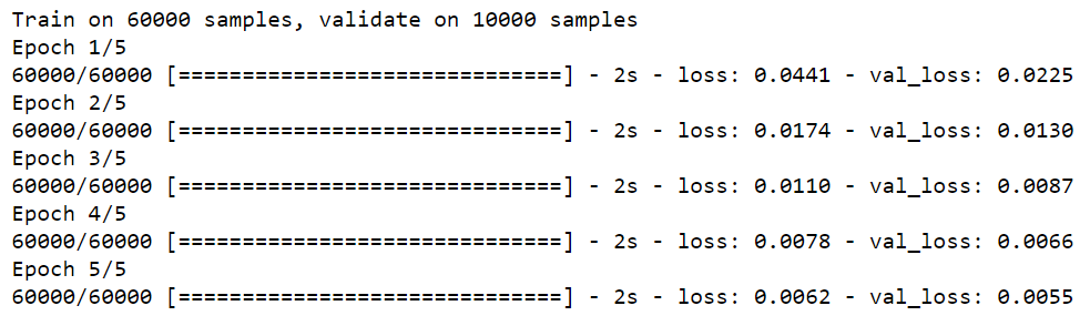
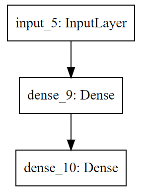
The first network is the most simple autoencoder. It has three layers : Input – encoded – decoded
input_size = 784
hidden_size = 64
output_size = 784
x = Input(shape=(input_size,))
h = Dense(hidden_size, activation='relu')(x)
r = Dense(output_size, activation='sigmoid')(h)

autoencoder = Model(inputs=x, outputs=r)
autoencoder.compile(optimizer='adam', loss='mse')
from IPython.display import SVG
from keras.utils.vis_utils import model_to_dot

SVG(model_to_dot(autoencoder).create(prog='dot', format='svg'))

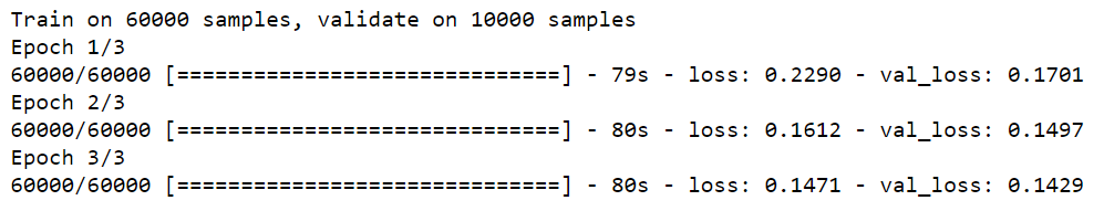
Train
epochs = 5
batch_size = 128

history = autoencoder.fit(X_train, X_train, batch_size=batch_size, epochs=epochs, verbose=1, validation_data=(X_test, X_test))
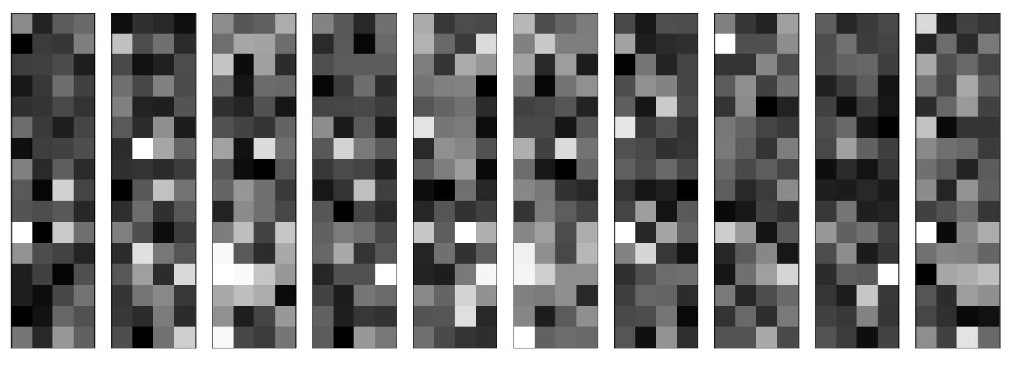
conv_encoder = Model(x, h)
encoded_imgs = conv_encoder.predict(X_test)

n = 10
plt.figure(figsize=(20, 8))
for i in range(n):
    ax = plt.subplot(1, n, i+1)
    plt.imshow(encoded_imgs[i].reshape(4, 16).T)
    plt.gray()
    ax.get_xaxis().set_visible(False)
    ax.get_yaxis().set_visible(False)
plt.show()
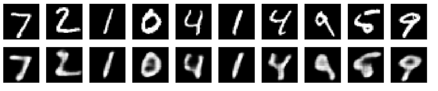
Predict on the test set
decoded_imgs = autoencoder.predict(X_test)
Plot
n = 10
plt.figure(figsize=(20, 6))
for i in range(n):
    # display original
    ax = plt.subplot(3, n, i+1)
    plt.imshow(X_test[i].reshape(28, 28))
    plt.gray()
    ax.get_xaxis().set_visible(False)
    ax.get_yaxis().set_visible(False)


    # display reconstruction
    ax = plt.subplot(3, n, i+n+1)
    plt.imshow(decoded_imgs[i].reshape(28, 28))
    plt.gray()
    ax.get_xaxis().set_visible(False)
    ax.get_yaxis().set_visible(False)

plt.show()

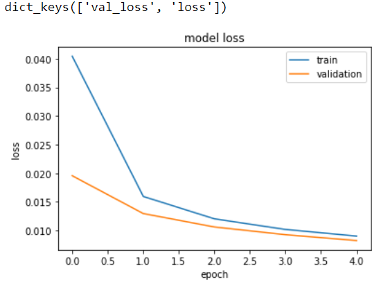
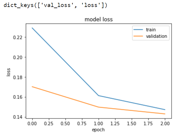
Plot the losses
print(history.history.keys())

plt.plot(history.history['loss'])
plt.plot(history.history['val_loss'])
plt.title('model loss')
plt.ylabel('loss')
plt.xlabel('epoch')
plt.legend(['train', 'validation'], loc='upper right')
plt.show()

Multilayer autoencoder
Create the network
We extend the idea of the first network to more layers
input_size = 784
hidden_size = 128
code_size = 64

x = Input(shape=(input_size,))
hidden_1 = Dense(hidden_size, activation='relu')(x)
h = Dense(code_size, activation='relu')(hidden_1)
hidden_2 = Dense(hidden_size, activation='relu')(h)
r = Dense(input_size, activation='sigmoid')(hidden_2)

autoencoder = Model(inputs=x, outputs=r)
autoencoder.compile(optimizer='adam', loss='mse')
from IPython.display import SVG
from keras.utils.vis_utils import model_to_dot

SVG(model_to_dot(autoencoder).create(prog='dot', format='svg'))

Train the network
epochs = 5
batch_size = 128

history = autoencoder.fit(X_train, X_train, batch_size=batch_size, epochs=epochs, verbose=1, validation_data=(X_test, X_test))

Predict on the test set
decoded_imgs = autoencoder.predict(X_test)
Plot
n = 10
plt.figure(figsize=(20, 6))
for i in range(n):
    # display original
    ax = plt.subplot(3, n, i+1)
    plt.imshow(X_test[i].reshape(28, 28))
    plt.gray()
    ax.get_xaxis().set_visible(False)
    ax.get_yaxis().set_visible(False)


    # display reconstruction
    ax = plt.subplot(3, n, i+n+1)
    plt.imshow(decoded_imgs[i].reshape(28, 28))
    plt.gray()
    ax.get_xaxis().set_visible(False)
    ax.get_yaxis().set_visible(False)

plt.show()

Plot the losses
print(history.history.keys())

plt.plot(history.history['loss'])
plt.plot(history.history['val_loss'])
plt.title('model loss')
plt.ylabel('loss')
plt.xlabel('epoch')
plt.legend(['train', 'validation'], loc='upper right')
plt.show()
Convolutional autoencoder
nb_classes = 10

(X_train, y_train), (X_test, y_test) = mnist.load_data()

X_train = X_train.reshape(X_train.shape[0], 28, 28, 1)
X_test = X_test.reshape(X_test.shape[0], 28, 28, 1)
X_train = X_train.astype("float32")/255.
X_test = X_test.astype("float32")/255.
print('X_train shape:', X_train.shape)
print(X_train.shape[0], 'train samples')
print(X_test.shape[0], 'test samples')

y_train = np_utils.to_categorical(y_train, nb_classes)
y_test = np_utils.to_categorical(y_test, nb_classes)
Create the network
This network does not take flattened vectors as an input but images
x = Input(shape=(28, 28,1))

# Encoder
conv1_1 = Conv2D(16, (3, 3), activation='relu', padding='same')(x)
pool1 = MaxPooling2D((2, 2), padding='same')(conv1_1)
conv1_2 = Conv2D(8, (3, 3), activation='relu', padding='same')(pool1)
pool2 = MaxPooling2D((2, 2), padding='same')(conv1_2)
conv1_3 = Conv2D(8, (3, 3), activation='relu', padding='same')(pool2)
h = MaxPooling2D((2, 2), padding='same')(conv1_3)


# Decoder
conv2_1 = Conv2D(8, (3, 3), activation='relu', padding='same')(h)
up1 = UpSampling2D((2, 2))(conv2_1)
conv2_2 = Conv2D(8, (3, 3), activation='relu', padding='same')(up1)
up2 = UpSampling2D((2, 2))(conv2_2)
conv2_3 = Conv2D(16, (3, 3), activation='relu')(up2)
up3 = UpSampling2D((2, 2))(conv2_3)
r = Conv2D(1, (3, 3), activation='sigmoid', padding='same')(up3)

autoencoder = Model(inputs=x, outputs=r)
autoencoder.compile(optimizer='adadelta', loss='binary_crossentropy')
from IPython.display import SVG
from keras.utils.vis_utils import model_to_dot

SVG(model_to_dot(autoencoder).create(prog='dot', format='svg'))
Train
epochs = 3
batch_size = 128

history = autoencoder.fit(X_train, X_train, batch_size=batch_size, epochs=epochs, verbose=1, validation_data=(X_test, X_test))
decoded_imgs = autoencoder.predict(X_test)
Plot
n = 10
plt.figure(figsize=(20, 6))
for i in range(n):
    # display original
    ax = plt.subplot(3, n, i+1)
    plt.imshow(X_test[i].reshape(28, 28))
    plt.gray()
    ax.get_xaxis().set_visible(False)
    ax.get_yaxis().set_visible(False)


    # display reconstruction
    ax = plt.subplot(3, n, i+n+1)
    plt.imshow(decoded_imgs[i].reshape(28, 28))
    plt.gray()
    ax.get_xaxis().set_visible(False)
    ax.get_yaxis().set_visible(False)

plt.show()
Plot the losses
print(history.history.keys())

plt.plot(history.history['loss'])
plt.plot(history.history['val_loss'])
plt.title('model loss')
plt.ylabel('loss')
plt.xlabel('epoch')
plt.legend(['train', 'validation'], loc='upper right')
plt.show()
Regularized autoencoder
Two types of regularization are described :
- Sparse autoencoder
- Denoising autoencoder
1. Sparse autoencoder
Create the network
input_size = 784
hidden_size = 32
output_size = 784
x = Input(shape=(input_size,))
h = Dense(hidden_size, activation='relu', activity_regularizer=regularizers.l1(10e-5))(x)
r = Dense(output_size, activation='sigmoid')(h)

autoencoder = Model(inputs=x, outputs=r)
autoencoder.compile(optimizer='adam', loss='mse')
from IPython.display import SVG
from keras.utils.vis_utils import model_to_dot

SVG(model_to_dot(autoencoder).create(prog='dot', format='svg'))
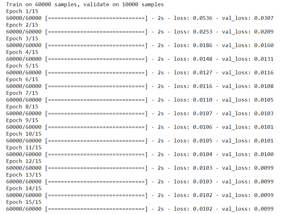
epochs = 15
batch_size = 128

history = autoencoder.fit(X_train, X_train, batch_size=batch_size, epochs=epochs, verbose=1, validation_data=(X_test, X_test))
Predict on the test set
decoded_imgs = autoencoder.predict(X_test)
Plot
n = 10
plt.figure(figsize=(20, 6))
for i in range(n):
    # display original
    ax = plt.subplot(3, n, i+1)
    plt.imshow(X_test[i].reshape(28, 28))
    plt.gray()
    ax.get_xaxis().set_visible(False)
    ax.get_yaxis().set_visible(False)


    # display reconstruction
    ax = plt.subplot(3, n, i+n+1)
    plt.imshow(decoded_imgs[i].reshape(28, 28))
    plt.gray()
    ax.get_xaxis().set_visible(False)
    ax.get_yaxis().set_visible(False)

plt.show()

Plot the losses
print(history.history.keys())

plt.plot(history.history['loss'])
plt.plot(history.history['val_loss'])
plt.title('model loss')
plt.ylabel('loss')
plt.xlabel('epoch')
plt.legend(['train', 'validation'], loc='upper right')
plt.show()

2. Denoising autoencoder
(X_train, _), (X_test, _) = mnist.load_data()

X_train = X_train.reshape(X_train.shape[0], 28, 28, 1)
X_test = X_test.reshape(X_test.shape[0], 28, 28, 1)

X_train = X_train.astype("float32")/255.
X_test = X_test.astype("float32")/255.
Create noisy data
noise_factor = 0.5
X_train_noisy = X_train + noise_factor * np.random.normal(loc=0.0, scale=1.0, size=X_train.shape)
X_test_noisy = X_test + noise_factor * np.random.normal(loc=0.0, scale=1.0, size=X_test.shape)

X_train_noisy = np.clip(X_train_noisy, 0., 1.)
X_test_noisy = np.clip(X_test_noisy, 0., 1.)
Create the network
x = Input(shape=(28, 28, 1))

# Encoder
conv1_1 = Conv2D(32, (3, 3), activation='relu', padding='same')(x)
pool1 = MaxPooling2D((2, 2), padding='same')(conv1_1)
conv1_2 = Conv2D(32, (3, 3), activation='relu', padding='same')(pool1)
h = MaxPooling2D((2, 2), padding='same')(conv1_2)


# Decoder
conv2_1 = Conv2D(32, (3, 3), activation='relu', padding='same')(h)
up1 = UpSampling2D((2, 2))(conv2_1)
conv2_2 = Conv2D(32, (3, 3), activation='relu', padding='same')(up1)
up2 = UpSampling2D((2, 2))(conv2_2)
r = Conv2D(1, (3, 3), activation='sigmoid', padding='same')(up2)

autoencoder = Model(inputs=x, outputs=r)
autoencoder.compile(optimizer='adadelta', loss='binary_crossentropy')
from IPython.display import SVG
from keras.utils.vis_utils import model_to_dot

SVG(model_to_dot(autoencoder).create(prog='dot', format='svg'))
Train the network
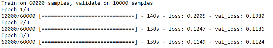
epochs = 3
batch_size = 128

history = autoencoder.fit(X_train_noisy, X_train, batch_size=batch_size, epochs=epochs, verbose=1, validation_data=(X_test_noisy, X_test))
decoded_imgs = autoencoder.predict(X_test_noisy)
Plot
n = 10
plt.figure(figsize=(20, 6))
for i in range(n):
    # display original
    ax = plt.subplot(3, n, i+1)
    plt.imshow(X_test_noisy[i].reshape(28, 28))
    plt.gray()
    ax.get_xaxis().set_visible(False)
    ax.get_yaxis().set_visible(False)


    # display reconstruction
    ax = plt.subplot(3, n, i+n+1)
    plt.imshow(decoded_imgs[i].reshape(28, 28))
    plt.gray()
    ax.get_xaxis().set_visible(False)
    ax.get_yaxis().set_visible(False)

plt.show()

Plot the losses
print(history.history.keys())

plt.plot(history.history['loss'])
plt.plot(history.history['val_loss'])
plt.title('model loss')
plt.ylabel('loss')
plt.xlabel('epoch')
plt.legend(['train', 'validation'], loc='upper right')
plt.show()

Valuable info. Lucky me I found your website by accident, and I’m shocked why this accident didn’t happened earlier! I bookmarked it.